
-
Basic Statistics
Basic Statistics
Probability Theory
Mutually Exclusive Events and Overlapping Events
Objective and Subjective Probabilities
Conditional (Posterior) Probability
Independent Events
Law of Total Probabilities
Bayes Theorem
Discrete Probability Distribution
Binomial Distribution
Poisson Distribution
Relationship between Variables
Covariance and Correlation
Joint Probability Distribution
Sum of Random Variables
Correlation and Causation
Simpson’s Paradox
Continuous Probability Distributions
Uniform Distribution
Exponential Distribution
Normal Distribution
Standard Normal Distribution
Approximating Binomial with Normal
t-test
Hypothesis Testing
Type I and Type II Errors
Statistical Significance and Practical Significance
Hypothesis Testing Process
One-Tailed — Known Standard Deviation
Two-tailed — Known Standard Deviation
One-Tailed — Unknown Standard Deviation
Paired t-test
ANOVA
Chi-Square (χ2)
Regression
Simple Linear and Multiple Linear Regression
Least Squares Error Estimation
Overview
Sample Size
Choice of Variables
Assumptions
Normality
Linearity
Dummy Variables
Interaction Effects
Variable Selection Methods
Issues with Variables
Multicollinearity
Outliers and Influential Observations
Coefficient of Determination (R2)
Adjusted R2
F-ratio: Overall Model
t-test: Coefficients
Goodness-of-fit
Validation
Process
Factor Analysis
- Basic Statistics
- Sampling
- Marketing mix Modelling
Coronavirus — What the metrics do not reveal?
Coronavirus — Determining death rate
- Marketing Education
- How to Choose the Right Marketing Simulator
- Self-Learners: Experiential Learning to Adapt to the New Age of Marketing
- Negotiation Skills Training for Retailers, Marketers, Trade Marketers and Category Managers
- Simulators becoming essential Training Platforms
- What they SHOULD TEACH at Business Schools
- Experiential Learning through Marketing Simulators
-
MarketingMind
Basic Statistics
Basic Statistics
Probability Theory
Mutually Exclusive Events and Overlapping Events
Objective and Subjective Probabilities
Conditional (Posterior) Probability
Independent Events
Law of Total Probabilities
Bayes Theorem
Discrete Probability Distribution
Binomial Distribution
Poisson Distribution
Relationship between Variables
Covariance and Correlation
Joint Probability Distribution
Sum of Random Variables
Correlation and Causation
Simpson’s Paradox
Continuous Probability Distributions
Uniform Distribution
Exponential Distribution
Normal Distribution
Standard Normal Distribution
Approximating Binomial with Normal
t-test
Hypothesis Testing
Type I and Type II Errors
Statistical Significance and Practical Significance
Hypothesis Testing Process
One-Tailed — Known Standard Deviation
Two-tailed — Known Standard Deviation
One-Tailed — Unknown Standard Deviation
Paired t-test
ANOVA
Chi-Square (χ2)
Regression
Simple Linear and Multiple Linear Regression
Least Squares Error Estimation
Overview
Sample Size
Choice of Variables
Assumptions
Normality
Linearity
Dummy Variables
Interaction Effects
Variable Selection Methods
Issues with Variables
Multicollinearity
Outliers and Influential Observations
Coefficient of Determination (R2)
Adjusted R2
F-ratio: Overall Model
t-test: Coefficients
Goodness-of-fit
Validation
Process
Factor Analysis
- Basic Statistics
- Sampling
- Marketing mix Modelling
Coronavirus — What the metrics do not reveal?
Coronavirus — Determining death rate
- Marketing Education
- How to Choose the Right Marketing Simulator
- Self-Learners: Experiential Learning to Adapt to the New Age of Marketing
- Negotiation Skills Training for Retailers, Marketers, Trade Marketers and Category Managers
- Simulators becoming essential Training Platforms
- What they SHOULD TEACH at Business Schools
- Experiential Learning through Marketing Simulators
Regression
As mentioned in Section Relationship between Variables, the covariance and correlation statistics provide a measure of the strength of the linear relationship between two variables.
Regression analysis is a technique which further examines the relationship between variables. It models the relationship between one or more independent variables (predictors or explanatory variables) and a dependent variable (response variable) and explains or predicts the outcome of the dependent variable, as a function of the independent variables.
The two basic types of regression are simple linear regression and multiple linear regression. Simple linear regression models the relationship as a linear function of one independent variable, whereas multiple regression uses two or more independent variables.
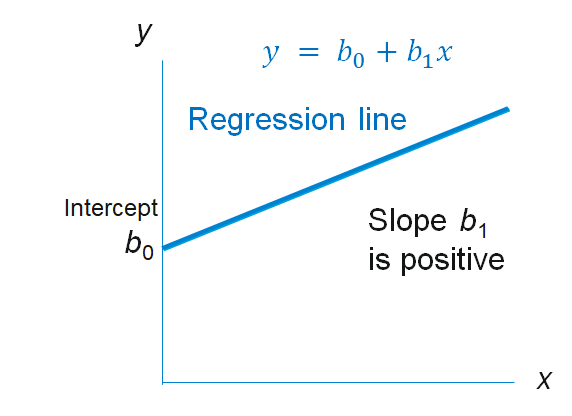
Simple linear regression (Exhibit 33.24) takes the following functional form: $$ y = b_0 + b_1x + e $$
Multiple linear regression takes the form:
$$ y = b_0 + b_1x_1 + b_2x_2 + b_3x_3 + ... + b_t x_t + e $$y: is the dependent or response variable.
x, xi: independent variables (predictors or explanatory variables).
b0: intercept.
bi: regression coefficient is the slope of the regression line.
e: error term
Once the relationship has been determined, the regression equation can be used to visualize, explain, and predict how the dependent variable responds to changes in the independent variables.
For instance, if you are studying the impact of consumer promotions, regression will explain how price discounts for an item and its competitors affect the sales of the item. It provides a measure for the discount price elasticity of demand and the cross-discount-price elasticity of demand, as well as the impact of displays and other in-store influences.
Based on this understanding, you can construct a “due to” analysis to explain the outcome of past marketing initiatives or develop a “what-if” analysis to predict or simulate the impact of proposed initiatives. These analyses are covered in Section Sales Decomposition and Due-To Analysis and Section What-if Analysis of Chapter Promotion.
Least Squares Error Estimation
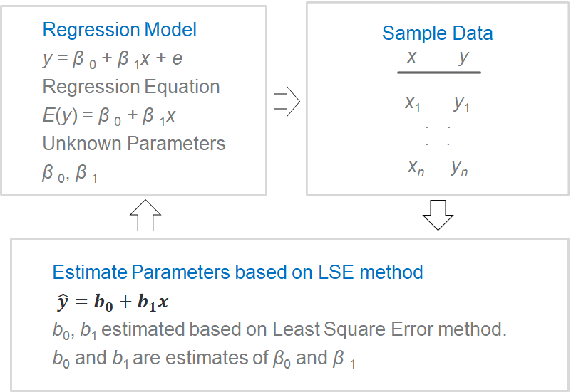
The approach to estimating the parameters for a regression equation is outlined in Exhibit 33.25. The intercept and coefficient estimates are based on the Least Squares Error (LSE) method where the criterion is to minimize the sum of the squared error (SSE) (actual – predicted): $$ min\sum(y_i-\hat y_i)^2 $$
yi: observed value.
ŷi: estimated value.
In the case of simple linear regression:
$$ SSE = \sum_{i=1}^n (y_i - \hat y_i )^2 = \sum_{i=1}^n [y_i - (b_0 + b_1 x_i)]^2 $$Via differentiation we can obtain the estimate for the regression coefficient:
$$b_1= \frac{\sum(x_i-\bar x)(y_i-\bar y)}{\sum(x_i - \bar x)^2}=\frac{SS_{xy}}{SS_{xx}}$$And, b0, the intercept:
$$ b_0=\bar y - b_1 \bar x $$As with simple regression, estimates for multiple linear regression are based on the LSE method. The parameters b1, b2, b3 etc. are called partial regression coefficients. They reveal the importance of their respective predictor variables, in driving the response variable.
Note: The partial contribution of each x-variable (as measured by its b-coefficient) may not agree in relative magnitude (or even sign) with the bivariate correlation between the x-variable and y (the dependent variable).
Regression coefficients vary with measurement scales. If we standardize (i.e., subtract the mean and divide by the standard deviation) y as well as x1, x2, x3, the resulting equation is scale-invariant:
$$ z_y = b_0^* + b_1^* × z_{x1} + b_2^* × z_{x2} + b_3^* × z_{x3}\, …$$Overview
While constructing a regression model, bear in mind that like any other market model, it should have a theoretical foundation, a conceptual framework. The selection of variables and their relationship should be based on concepts and theoretical principles.
The regression equation depicts the relationship between dependent and predictor variables, in terms of importance or magnitude, as well as direction.
The regression coefficients denote the relative importance of their respective predictor variables, in driving the response variable. The coefficient b1 for instance, represents the amount the dependent variable y is expected to change for one unit of change in the predictor x1, while the other predictors in the model are held constant.
The linear model is theoretically unsound for predicting sales (and most other marketing variables) because it suggests that sales can increase indefinitely. However, from a practical standpoint, a linear model can provide a good approximation of the true relationship over a small operating range, e.g., a + 15% change in a predictor such as price.
Nonlinear structural models can be transformed into estimation models that are linear in parameters by applying transformation functions. The advantage of doing this is that the parameters of the original nonlinear model can be estimated using linear-regression techniques.
For instance, consider the multiplicative form, which is widely used in marketing mix models such as NielsenIQ’s Scan*Pro:
$$ y=e^α x_1^{β_1} x_2^{β_2} x_3^{β_3}\,…$$This nonlinear structural model can be transformed into an estimation model that is linear in parameters by taking logarithms on both sides.
Sample Size
The size of the sample determines the reliability, the extent that the regression analysis result is error free. It determines the statistical power of the significance testing, as well as the generalizability, i.e., the ability to apply the result to the larger population.
As a thumb rule, 15 to 20 observations are required for each independent variable. If the sample is constrained, a bare minimum of 5 observations are required for each independent variable, provided there are at least 20 observations for simple regression, and 50 for multiple regression.
Small samples can detect only the stronger relationships. Moreover, if the ratio of observations to parameters is below norm, you run the risk of “overfitting” – making the results too specific to the sample, thus lacking generalizability. Increasing the degrees of freedom improves generalizability and reliability of the result.
Choice of Variables
The choice of variables is crucial to the validity and utility of a regression model.
The omission of relevant independent variable can severely distort the findings, particularly when the variable relates to a distinct influence, yet coincides (correlates) with some other independent variable.
For example, in Singapore, consumer promotions of some soft drink brands occur mainly during the Hungry Ghost festival. If the festive seasonality is not incorporated into the regression model, the discount price elasticity of these brands is greatly exaggerated as they soak up the impact of the festive season.
The inclusion of irrelevant variables is also a concern. It reduces the model’s parsimony and may also mask or replace the effects of more useful variables.
A separate issue pertains to errors in the measurement of variables, missing data points for instance. Where it is necessary to include the data, analyst make use of a variety of techniques to clean data and incorporate missing information.
Assumptions
There are a number of underlying assumptions about the dependent and independent variables, and their relationship, which affect the statistical procedures such as LSE and significance tests used for linear regression. These assumptions, listed here, need to be tested at the different stages of the regression process.
Normality: Variables and their combination are assumed to follow the normal distribution.
Linearity is assumed, as is evident from the name (linear regression).
Homoscedasticity: Variance of dependent variable should not vary across range of predictor variables.
Residuals (errors, i.e., predicted minus observed values) are assumed to be independent. The prediction errors should be uncorrelated, otherwise it suggests some unexplained, systematic relationship in the dependent variable.
Normality
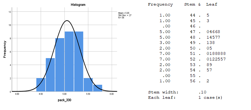
Exhibit 33.26 Histogram and Stem & Leaf plot reveals the shape of the distribution. The Stem & Leaf plots also enumerates the actual values. (Source: SPSS).
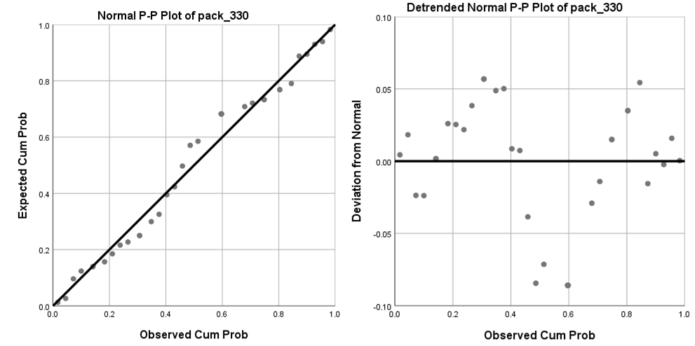
Exhibit 33.27 The normal probability plot and the de-trended normal probability plot. (Source: SPSS).
The dependent and independent variables are assumed to follow normal distribution. Furthermore, in the case of multiple regression, this assumption is also applicable to the combination of variables.
If their distributions vary substantially from the normal distribution, the F test, which assesses the overall regression, and the t-test, which assesses statistical significance of the coefficients, may no longer remain valid. These tests assume that the residuals are distributed normally.
Univariate normality can be visually examined through the histogram and the stem & leaf plot (Exhibit 33.26), though this may be problematic for smaller samples. The normal probability plot, Exhibit 33.27, is a more reliable check. This compares the cumulative distribution of the data with that for a normal distribution. If data is normal, it is scattered close to the diagonal which represents the theoretical normal distribution.
Additionally, the Kurtosis statistic tests for “peakedness” or “flatness” of the data, and the skewness statistic is a measure for skewness.
Linearity
Simple and multiple linear regression are linear by definition. Moreover, the correlation measures that these techniques are based on, represent only the linear association between variables.
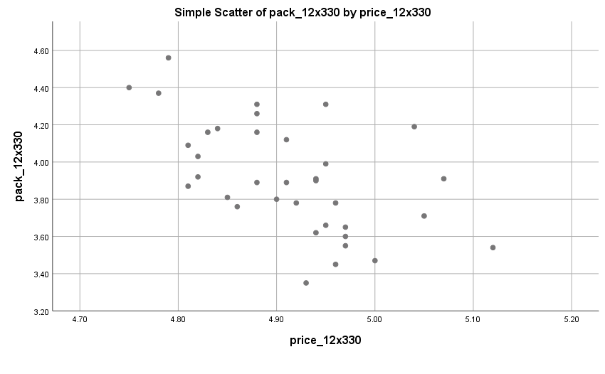
Linearity may be visually examined via scatterplots such as the one shown in Exhibit 33.29. Alternatively, for a more accurate assessment, you could run a simple regression analysis and examine the pattern of residuals.
Nonlinear relationship can be made linear in parameters by transforming one or more of the variables.
Common approaches include,for relatively flat distributions, the inverse transformation 1/x or 1/y, and for positively skewed distributions distribution, square root transformation: $$x_{new}=\sqrt{x_{old}},$$
And log, for negatively skewed distribution:
$$x_{new}= log(x_{old}).$$New variables may be created to represent the nonlinear portion of the relationship. Polynomials (x2 or x3) for instance, are power transformations of an independent variable that add a non-linear component:
- x1 (power = 1): linear.
- x2 (power = 2): quadratic. Single inflection point.
- x3 (power = 3): cubic. Two inflection points.
If the relationship is known to be nonlinear with inflection points, a common practice is to start with the linear component, and then sequentially add higher-order polynomials till there is no significant additional improvement in the fit (R2). The t-test would confirm whether or not the additional terms are significant.
Dummy Variables
When an independent variable is nonmetric (e.g., seasonality), and has k (two or more) categories, it can be represented by k-1 dummy variables.
For example, the coding of in-store causal influences like display and co-op advertising can be captured with the use 3 dummy variables:
- Display only. (No co-op): D1=1, D2=D3=0.
- Co-op, no display: D2=1, D1=D3=0.
- Display + co-op: D3=1, D1=D2=0.
- The 4th option, no display and no co-op, is represented by D1=D2=D3=0.
The impact of dummy variables is reflected in the change of intercept (b0). For instance, consider the relationship between sales and discount price. The x-coefficient (b1 = discount price elasticity) remains unchanged when there is a display. The impact of an in-store display is reflected in an incremental lift in sales, referred to as uplift.
Interaction Effects
Intended to achieve common imperatives, the elements of the marketing mix often interact synergistically to produce an effect greater than the sum of their individual effects.
Take consumer promotions for instance. Discounts, displays and co-op ads, often have a synergistic impact lifting sales more than the sum of their individual impact on sales.
Similarly, theme advertising strengthen a brand’s equity, resulting in the lowering of consumers’ sensitivity to changes in price.
These interaction effects where one element of the marketing mix affects the sensitivity of one or more other elements, can be captured in response functions by the inclusion of an additional term, x1 × x2, formed by the product of the two variables that interact.
$$ y = b_0 + b_1 x_1 + b_2 x_2 + b_3 x_1 x_2 $$In this example, the overall effect of x1 for any value of x2 is equal to: b1-total = b1 + b3 x2.
To determine the presence of the moderator effect (b3x1x2), compare the unmoderated R2 with the moderated R2. A statistically significant difference would imply the existence of the interaction effect between the variables.
Variable Selection Methods
As mentioned, the choice of variables is a crucial decision. The omission of relevant, important variables can distort the findings. The inclusion of irrelevant variables on the other hand, reduces model parsimony, and may also mask or replace the effects of more useful variables.
Once an initial set of variables has been listed, some of them may turn out to be less important, not contribute significantly to the relationship.
For example, in the analysis of promotions, the sale of an item depends on the discounted price of that item (discount price elasticity) as well as the discounted price of competing items (discounted cross-price elasticity). It will turn out that some competitor items do compete strongly, and their prices are included as variables in the final model, whereas the prices of other items are not having a significant impact, and they are removed from the model.
There are a variety of approaches leading to the final selection of variables. Some of these are discussed here.
The confirmatory approach is one where the analyst specifies the variables. Typically, one would use a variety of other methods, arrive at some conclusions, and then confirm the variables that you want to deploy in the regression.
Another method commonly found in statistical packages is called stepwise regression. It follows this sequence of steps:
- At the start, dependent variable (y) is regressed with the most highly correlated predictor variable (x1): $$ y = b_0+b_1 x_1 $$
- Next, the predictor (x2) with highest partial correlation, is added to the model: $$ y = b_0+b_1 x_1+b_2 x_2 $$
- After each additional variable is added, the algorithm examines the partial F value for the previous variable(s) (x1). If the variable no longer makes a significant contribution, given the presence of the new variable, it is removed.
- Steps 2 and 3 are repeated with remaining independent variables, till all are examined, and a “final” model emerges.
Sometimes the coefficients of one or two variables in the final model may not be meaningful; the direction of the relationship may be nonsensical. Normally this occurs for variables that have relatively low contribution to the relationship, and they can be removed.
Another approach referred to as the forward regression is similar to the stepwise method. It adds independent variables progressively as long as they make contributions greater than some threshold level. However, unlike stepwise estimation, once selected, variables are not deleted at any subsequent stage.
Yet another approach, backward regression, is essentially forward regression in reverse. It starts with all possible independent variables in the model, and sequentially deletes those which make contributions below some threshold value.
These diverse model selection procedures, which are automated in statistical packages like R, SAS and SPSS, are useful for variable screening.
In applications such as data mining, where the association between variables is often unknown and needs to be explored, these techniques help unearth promising relationships.
Issues with Variables
Issues pertaining to variables need to be addressed to ensure the outcome is a model that is statistically significant and theoretically sound.
Regression can ascertain relationships, but not the underlying causal mechanism. So, first and foremost, models must remain true to their theoretical foundation. We must ensure that the coefficients are meaningful; that their expected sign and magnitude are conceptually correct.
A subtle problem can arise due to the stepwise estimation process. Since it takes one variable at a time, if a pair (xi, xj) collectively explain a significant proportion of the variance, they will not be selected by the stepwise method, if by themselves, neither is significant.
Another issue, multicollinearity or the correlation among independent variables may make some variables redundant. This needs to be assessed, since in the selection process, it is likely that after one is included, the others will not be included.
While multicollinearity masks relationships that are not needed for predictive purposes, it does not reflect on their relationship with the dependent variable. This is discussed in the next section.
The inclusion of variables with low multicollinearity with the other independent variables, and high correlation with the dependent variable, increases the overall predictive power of a model.
Multicollinearity
Collinearity is the correlation between two independent variables, and multicollinearity is the correlation between three or more independent variables. The terms, however, are often used interchangeably.
Multicollinearity reduces the predictive power of an independent variable by the extent to which it is associated with other independent variables. As the correlation increases, the proportion of the variance explained by each independent variable decreases, while their shared contribution increases.
An extreme example of multicollinearity would be duplicate variables, for instance advertising spend in dollars and in ‘000 dollars. These two variables are essentially identical, and one should be removed.
On the other hand, if one of the variables is GRP and the other is spend in dollars, in that case the analyst should pick the one that has the greater predictive power. (In theory, that ought to be GRP, if the dependent variable is advertising awareness or sales).
Finally, consider Brand Equity research. Of the large number of attributes that relate to brand equity, many are correlated. For instance, value for money, low price, attractive promotions and house brands.
The approach in this case is to club variables together to form factors, or composite variables. The dependent variable is then regressed with the factors; the regression coefficients reveal the importance of each factor, and the factor loading reveals the importance of each attribute or independent variable.
To sum up, sometimes factor analysis and other means of combining variables into summated scales, can effectively address multicollinearity. In other instances, one or more of the variables may be redundant.
Outliers and other Influential Observations
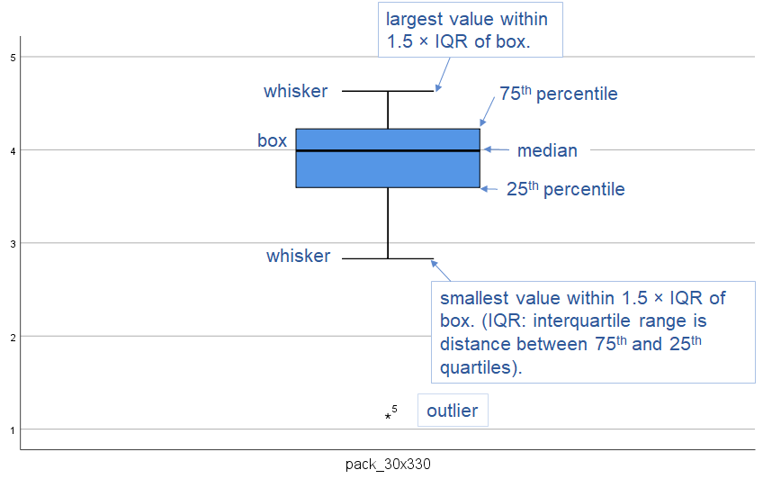
Exhibit 33.30 Box and Whiskers plot. This indicates whether distribution is skewed and reveals outliers, i.e., values lying beyond the whiskers (data point #5).
An outlier is an observation that is distant from other observations. It may result from measurement error; in which case it should be discarded. Or it may be indicative of a heavy-tailed population distribution, which then violates the assumption of normality.
Box and whisker plots such as the one shown in Exhibit 33.30, reveal outliers in a univariate assessment. For pairs of variables, outliers appear as isolated points on the outskirts of scatterplots. For more than 2 variables, statistical techniques such as Mahalanobis D2 may be used for detecting outliers.
Influential observations are any observations, outliers included, that have a disproportionate effect on the regression results. These need to be carefully examined and should be removed, unless there is a rationale for retaining them.
Coefficient of Determination (R2) — How close is the fit?
Coefficient of Determination (R2) represents the proportion of the variance of a dependent variable that is explained by the predictor(s).
The sum of squared deviations, ∑(yi − ȳ)2 (SStot), is an unscaled, or unadjusted measure of dispersion or variability. When scaled for the number of degrees of freedom, it becomes the variance.
Partitioning of the sum of squared deviations, allows the overall variability in the data to be ascribed to that explained by the regression (SSreg), and that not explained by the regression, i.e., the residual sum of squares, (SSres).
$$ SS_{tot} = SS_{reg} + SS_{res} $$ $$ \text{Total SS = Explained SS + Residual SS} $$ $$ \sum(y_i - \bar y)^2=\sum(\hat y_i - \bar y)^2 + \sum (y_i - \hat y_i )^2 $$SStot: Total sum of squared deviations.
SSreg: Explained sum of squared deviation.
SSres: Residual (error) sum of squares.
Coefficient of Determination (R2) is the proportion of the variance in the dependent variable that is predictable from the independent variables:
$$R^2=\frac{SS_{reg}}{SS_{tot}}$$This is a commonly used statistic to evaluate model fit; it is an indicator of how well the model explains the movement in the data. For instance, an R2 of 0.8 means that the regression model explains 80% of the variability in the data.
Radj2: Adjusted R2
R2 always increases when explanatory variables are added to a model. As such it can create the illusion of a better fit as more terms are added.
Radj2 adjusts for number of explanatory terms in a model relative to the number of data points. Unlike R2, the Radj2 increases only when the increase in R2 (due to inclusion of variable) is more than one would expect to see by chance.
$$ R_{adj}^2 = 1 – \frac{(1 – R^2)× (n – 1)}{n – k – 1}$$Where k is the number of explanatory variables, and n is sample size.
As explanatory variables are added to a regression in order of importance, the point before Radj2 starts to decrease, is where the stepwise selection of variables should conclude.
F-ratio: Statistical Significance of the Overall Model
The F-ratio, which follows the F-distribution, is the test statistic to assess the statistical significance of the overall model. It tests the hypothesis that the variation explained by regression model is more than the variation explained by the average value (ȳ).
$$ F =\frac{SS_{reg}/df_{reg}}{SS_{res}/df_{res}} $$ $$ = \frac{R^2/k}{(1-R^2)/(n-k-1)}$$Where:
k is the number of explanatory variables, and n is sample size.
SSreg: Explained sum of squared deviation.
SSres: Residual (error) sum of squares.
dfreg: Degrees of freedom (regression) = number of estimated coefficients including intercept − 1 = number of explanatory variables (k).
dfres: Degrees of freedom (residual) = sample size (n) − (k+1).
R2: Coefficient of Determination (R2) is the proportion of the variance in the dependent variable that is predictable from the independent variable.
t-test: Statistical Significance of the Coefficients
Since the coefficients in the regression represent key parameters such as elasticities and cross-elasticities of demand, it is important that we test their statistical significance.
The t-test is used for this purpose. For each coefficient, it tests that the coefficient differs significantly from zero value.
Consider the regression model: $$ y = b_0+b_1 x_1+b_2 x_2+b_3 x_3 \,…$$
For the coefficient b1, in the above equation:
Null hypothesis H0: b1 = 0
Alternative hypothesis HA: b1 <> 0
Relevant test statistic is t = b1 /σb1, where σb1 is the standard error of b1.
Relevant distribution is the t-distribution, with degrees of freedom = n − (k + 1). Where k is the number of explanatory variables, and n is sample size.
Similar tests are run for b2, b3 … to determine the individual significance of X2 and X3 in the model.
Goodness-of-fit: Desirable Properties of a Regression Model
In interpreting the quality of a regression model, the following aspects are taken into consideration.
High adjusted R2: R2 is proportion of variation in the dependent variable explained by the independent variables. Radj2 adjusts for number of explanatory terms in a model relative to the number of data points (i.e., df associated with the sums of squares).
Significant F-statistic: The null hypothesis that all coefficients (b1, b2 …) are zero can be conclusively rejected
Significant t-statistics: The individual coefficients are statistically significant.
Residuals are random, normally distributed, with mean 0, and their variance does not vary significantly, over the values of the independent variables.
Validation
Validation, or more specifically, cross-validation is a method of assessing how well the regression can be generalized.
One approach it to retain a portion of the original data for validation purposes and use the rest to construct the model. Once the model is finalized, the estimated parameters are used to predict the out-of-sample data.
The model’s validity may be assessed by comparing the out-of-sample mean squared error (the mean squared prediction error), with the in-sample mean square error. If the out-of-sample mean squared error is substantially higher, that would imply deficiency in the model’s ability to predict.
Process
To summarize, here is the sequence of steps to be followed in the development of a regression model.
- Research Objective stems from the marketing objective. It determines which dependent variables or responses need to be predicted, and/or what needs to be explained.
- Sample: The sample size should be adequately large to ensure statistical power and generalizability of the regression.
- Model design: Choose the dependent and plausible explanatory variables. Check
assumptions:
- Normality
- Linearity
- Homoscedasticity
- Independence of the error terms.
- Transformations, in case some assumptions are not met.
- Dummy variables to cater for nonmetric variables.
- Polynomials required if curvilinear relationships exist.
- Interaction terms required if there are moderator effects.
- Run the model. Variable Selection is usually a combination of methods such as confirmatory, stepwise estimation, forward regression and backward regression.
- Examine Results: Output need to be thoroughly examined in the context of the following:
- Issues: Influential observations. Check for multicollinearity.
- Practical Significance: Is it theoretically sound? Are the signs and magnitude of coefficient meaningful?
- Statistical Significance:
- Radj2: Adjusted coefficient of determination.
- F-ratio: Standard error of estimation.
- t-test: Statistical significance of regression coefficients.
- Residuals: Ensure that residuals meet required criteria.
- Validation: Cross-validate the regression to assess how well the model can be generalized.
Previous Next
Use the Search Bar to find content on MarketingMind.
Marketing Analytics Workshop
In an analytics-driven business environment, this analytics-centred consumer marketing workshop is tailored to the needs of consumer analysts, marketing researchers, brand managers, category managers and seasoned marketing and retailing professionals.
Digital Marketing Workshop

Unlock the Power of Digital Marketing: Join us for an immersive online experience designed to empower you with the skills and knowledge needed to excel in the dynamic world of digital marketing. In just three days, you will transform into a proficient digital marketer, equipped to craft and implement successful online strategies.


Contact | Privacy Statement | Disclaimer: Opinions and views expressed on www.ashokcharan.com are the author’s personal views, and do not represent the official views of the National University of Singapore (NUS) or the NUS Business School | © Copyright 2013-2024 www.ashokcharan.com. All Rights Reserved.